Week 6: July 07 ~ July 13
Preliminaries
This week, I focused on understanding and analyzing the dataset collected last week (week-05) using the follow-line The dataset includes images paired with corresponding linear (v) and angular (w) velocity values, which are essential for training deep learning models for autonomous control. I collected 84,969 data entries, each consisting of an image paired with corresponding action commands—specifically, linear velocity (v) and angular velocity (w). It helps a better understanding of the structure and distribution of the dataset and identifies imbalanced categories that may affect model performance.
To better understand the distribution of control commands and support classification-based training approaches, I began by analyzing and categorizing both linear (V) and angular (W) velocities into discrete classes. I also created visualizations to identify patterns, detect imbalance, and guide potential resampling strategies.
Objectives
- Understand the Distribution of Control Commands
- Categorize Velocities
- Visualize the Dataset
- Identify Imbalanced Categories
Execution
Categorization of Angular Velocity (w)
I categorized the angular velocity (w) values into five discrete classes based on the turning direction and intensity. This approach helps the model focus on steering behaviors rather than predicting exact floating-point values.
Here are the five categories:
- Sharp Left
- Left
- Straight
- Sharp Right
- Right
Angular Velocity (w) Descriptions
| Statistic | Value |
|---|---|
| Count | 84,969 |
| Mean | -0.029841 |
| Standard Deviation (std) | 0.376109 |
| Minimum (min) | -3.5 |
| Maximum (max) | 3 |
| 25th Percentile | -0.12933 |
| Median (50%) | -0.00237 |
| 75th Percentile | 0.09748 |
We can see the maximum and minimum values of the
angular velocity are -3.5 and
3.0. We divided the range into five
categories.
Angular Velocity (w) Categories
| Category | Range (W) | Description |
|---|---|---|
| Sharp Right | W ≤ -1.0 | Hard turn right |
| Right | -1.0 < W ≤ -0.1 | Slight right |
| Straight | -0.1 < W < 0.1 | No turn |
| Left | 0.1 ≤ W < 1.0 | Slight left |
| Sharp Left | W ≥ 1.0 | Hard turn left |
Angular velocity (W): Data distribution among the categories
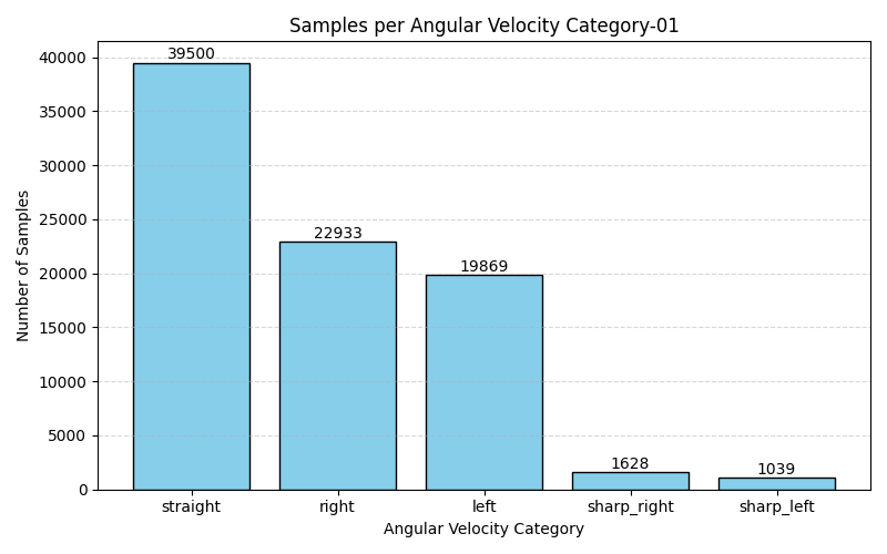 Entries per categories
Image Samples per categories
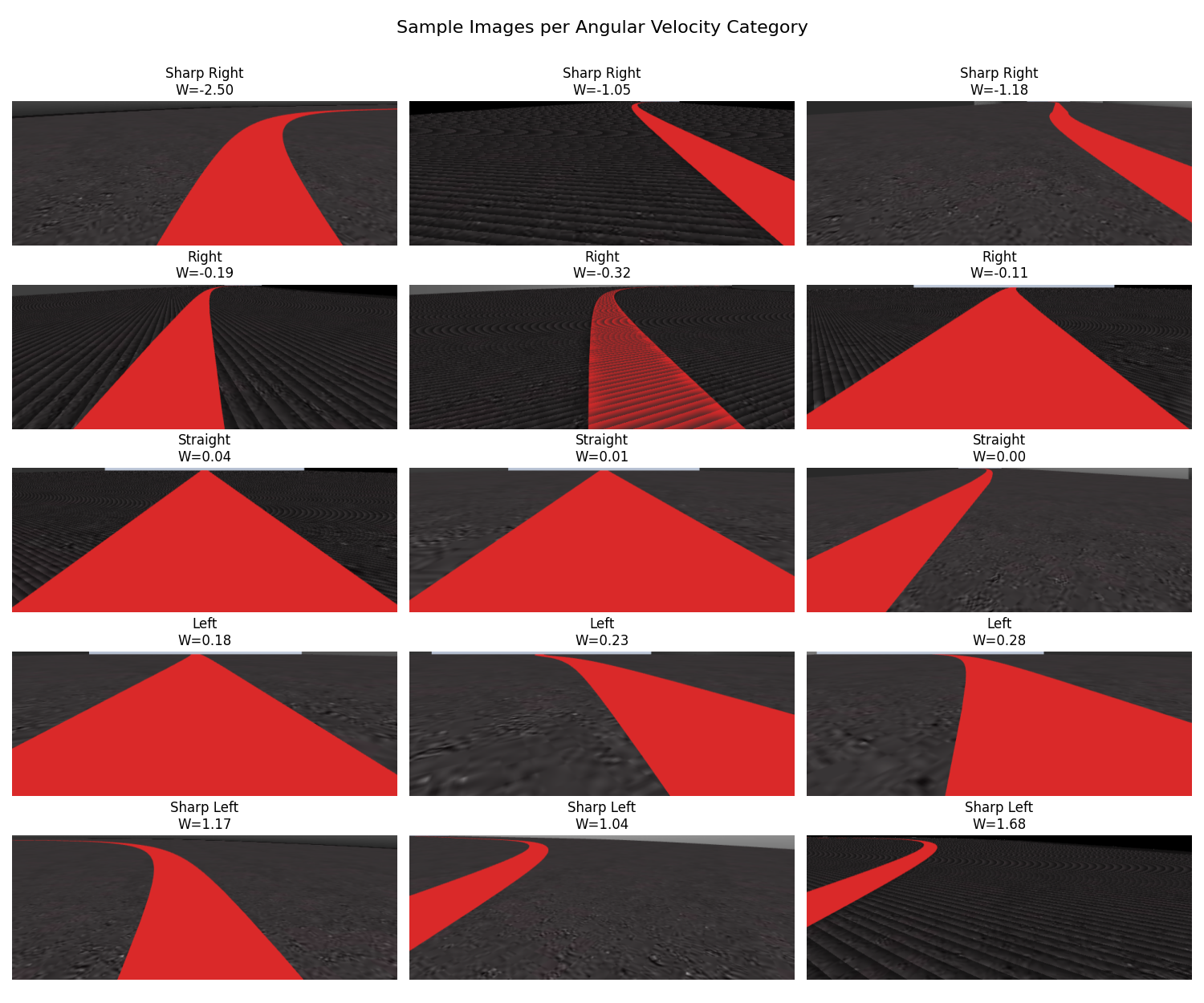 image Samples per categories
Categorization of Linear Velocity (v)
I categorized the linear velocity (v) values into four(4) discrete classes based on speed and direction. This approach helps the model focus on speed behaviors rather than predicting exact floating-point values.
The linear velocity values in the dataset range from
5 to 11. I divided them into four categories, each
with a range of 1.5 units. (Calculated as:
(11 - 5) / 4 = 1.5)
Here are the four(4) categories:
- Slow
- Moderate
- Fast
- Very Fast
Linear Velocity (v) Descriptions
| Statistic | Value |
|---|---|
| Count | 84,969 |
| Mean | 8.122210 |
| Standard Deviation (std) | 1.954871 |
| Minimum (min) | 5.000000 |
| Maximum (max) | 11.000000 |
| 25th Percentile | 6.440000 |
| Median (50%) | 8.648000 |
| 75th Percentile | 9.752000 |
Linear Velocity (v) Categories
| Category | Description | Velocity Range (v) |
|---|---|---|
| slow | Lowest speed | v ≤ 6.5 |
| moderate | Moderate speed | 6.5 < v ≤ 8.0 |
| fast | Fast speed | 8.0 < v ≤ 9.5 |
| very_fast | Very fast | v > 9.5 |
Linear velocity (v): Data distribution among the categories
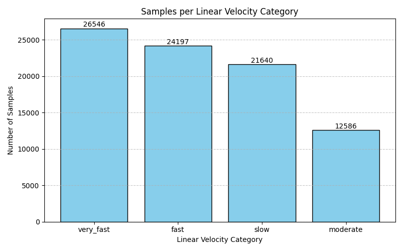 Entries per categories
Frequency of linear velocity (v) vs angular velocity (w)
The analysis indicates how often combinations of linear and angular velocities occur.
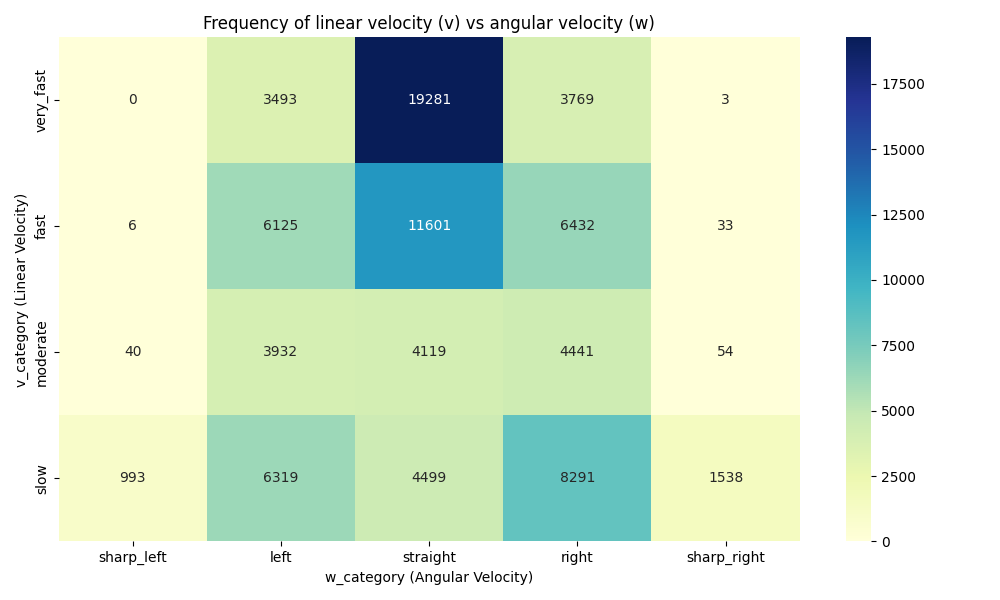 Frequency of linear velocity (v) vs angular
velocity (w)
Frequency of linear velocity (v) vs angular
velocity (w)
References
Enjoy Reading This Article?
Here are some more articles you might like to read next: