Week 2
After a basic prototype for the human detection exercise was ready, I decided it was the best time to add the model benchmarking features to the exercise. Adding benchmarking related features had always been in my mind since the beginning considering the importance it would hold in view of the exercise. It was now time to plan on going about it. I was still very naive with the technical knowledge required to implement benchmarking for object detection models. Nevertheless, I started referring to some pretty solid online resources, which helped me get started with it.
Added model analyzer
Adding cool and innovative tools which can make the use of the exercise more productive for the end user has always been my top priority. There have often been cases with me in the past where I have faced errors while trying to make my Deep Learning model work for the respective task. A majority of the times it had got something to do with a problem related to the mismatch of input shapes to some layer or an ambiguity in the architecture. For some complex models it can be a headache to refer back to the code again and again checking for mistakes. For this reason, I started searching for a tool which could help us visualize the model in real time.
I started off with implementing the build in model analysis feature provided with the ONNX library, which looked something like:
import onnx
import os

# load the ONNX model
model_path = os.path.join('test_model', 'single_relu.onnx')
onnx_model = onnx.load(model_path)

print('The model is:\n{}'.format(onnx_model))
# output

The model is:
ir_version: 3
producer_name: "backend-test"
graph {
  node {
    input: "x"
    output: "y"
    name: "test"
    op_type: "Relu"
  }
  name: "SingleRelu"
  input {
    name: "x"
    type {
      tensor_type {
        elem_type: 1
        shape {
          dim {
            dim_value: 1
          }
          dim {
            dim_value: 2
          }
        }
      }
    }
  }
  output {
    name: "y"
    type {
      tensor_type {
        elem_type: 1
        shape {
          dim {
            dim_value: 1
          }
          dim {
            dim_value: 2
          }
        }
      }
    }
  }
}
opset_import {
  version: 6
}
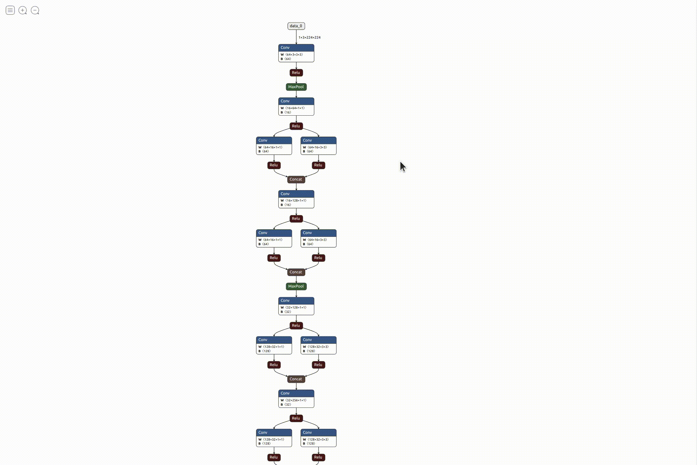
This was fine from an analysis point of view, but to be honest it didn’t really solve my purpose of visualization as it was only slightly better than referring to the raw code. I wanted something more interactive, easy to refer to and visually appealing. After searching for something similar, I found this really cool open source visualizer for neural network, deep learning, and machine learning models called Netron. It was perfect for what I needed, so I started working on integrating it with the exercise. Luckily, it also came with an API to run it as a python server on the local machine. I referred to the instructions and added it to the exercise code. After everything was in place, it was pretty simple running the visualizer.
def visualizeModel(self, raw_dl_model):
    raw_dl_model = raw_dl_model.split(",")[-1]
    raw_dl_model_bytes = raw_dl_model.encode('ascii')
    raw_dl_model_bytes = base64.b64decode(raw_dl_model_bytes)
    try:
        with open(self.aux_model_fname, "wb") as f:
            f.write(raw_dl_model_bytes)
        netron.start(self.aux_model_fname)
    except Exception:
        exc_type, exc_value, exc_traceback = sys.exc_info()
        self.console.print(str(exc_value))
        self.console.print("ERROR: Model couldn't be loaded to the visualizer")
Working on model benchmarking
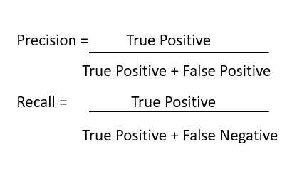
Like I mentioned before I was new to object detection benchmarking. Previously I had worked only on evaluating classification based ML models based on Accuracy, Precision, Recall or an F1- Score. I started referring to resources on the internet to guide me on this.
Basically, the objective of an object detection models is to perform:
- Classification: Identify if an object is present in the image and the class of the object
- Localization: Predict the co-ordinates of the bounding box around the object when an object is present in the image. Here we compare the co-ordinates of ground truth and predicted bounding boxes
This means we need to evaluate the performance of both classification as well as localization of using bounding boxes in the image. This is where the concept of Intersection over Union (IoU) comes in.
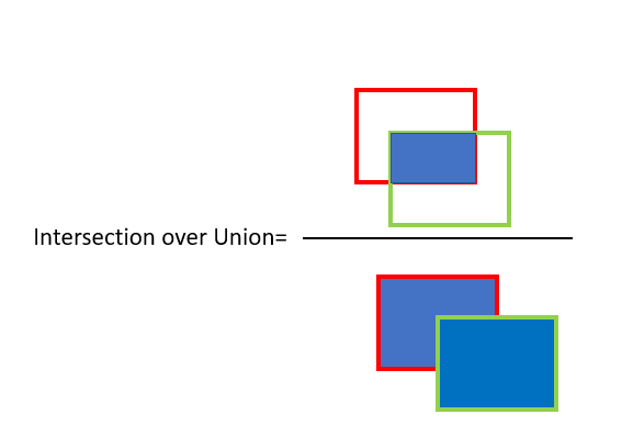
Intersection over Union (IoU)
IoU computes intersection over the union of the two bounding boxes; the bounding box for the ground truth and the predicted bounding box. An IoU of 1 implies that predicted and the ground-truth bounding boxes perfectly overlap. We can set a threshold value for the IoU to determine if the object detection is valid or not not. Based on this and the corresponding ground truth value of the detection, we can classify wether it’s True Positive(TP), False Positive(FP) or False Negative(FN).
The idea was to then calculate precision and recall based on the values of TP, FP and FN obtained for detections per image. I kind of started a bottom up approach for this to check it’s feasibility. What I mean to say is that I started to build directly from calculating the precision, recall part itself assuming that down the line I would eventually implement the IOU part and subsequent classification of detections into the above categories. Of course, this also includes finding and preprocessing an appropriate benchmarking data set.
def calc_precision_recall(image_results):
    """Calculates precision and recall from the set of images
        img_results (dict): formatted like:
            {
                'img_id1': {'true_pos': int, 'false_pos': int, 'false_neg': int},
                'img_id2': ...
                ...
            }
    Returns:
        tuple: of floats of (precision, recall)
    """
    true_positive=0
    false_positive=0
    false_negative=0
    for img_id, res in image_results.items():
        true_positive +=res['true_positive']
        false_positive += res['false_positive']
        false_negative += res['false_negative']
        try:
            precision = true_positive/(true_positive+ false_positive)
        except ZeroDivisionError:
            precision=0.0
        try:
            recall = true_positive/(true_positive + false_negative)
        except ZeroDivisionError:
            recall=0.0
    return (precision, recall)
As of now I am assuming that I have received the image_results parameter from a magic source. Well, this magic source would be no magic but something we would implement down the line as part of our benchmarking code only. Here’s how I plan this would happen:
- Let’s assume we already have an annotated ground truth dataset.
- Feed the dataset frame by frame to the evaluation inference code and save the detections in an appropriate manner.
- Feed the detections and the corresponding ground truth values to the Intersection Over Union (IOU) code, which based on a specified IOU threshold, will then classify each detection per image into one of the 3 catagories i.e True Positive(TP), False Positive(FP) or False Negative(FN). After this it would accumulate these values per image in a form like:
img_results = { 'img_id1': {'true_pos': int, 'false_pos': int, 'false_neg': int}, 'img_id2': {'true_pos': int, 'false_pos': int, 'false_neg': int}, ...... } - We can then feed the
img_resultsto thecalc_precision_recall()function. - Based on the calculated precision/recall values, we can then plot the corresponding precision VS recall graph and also find out the Average Precision of the model.
Of course, all this is just a tentative vision of how I plan to implement the benchmarking process. It may change based on what difficulties I face and wether I can find appropriate resources for the same.
Now, before moving ahead with all this, it was important to first collect an appropriate dataset to suit our needs.
Collecting Benchmarking Dataset
I referred to the following datasets before choosing the final one:
-
Caltech Pedestrian Detection Benchmark - Overall this was a pretty good dataset. The video sequence for this was in a binary .seq type file, whereas the corresponding annotations were in a .vbb file. However, the dataset website didn’t provide any matlab code to extract the annotations from the .vbb file. I referred to the internet for the same but couldn’t find anything legit.
-
CrowdHuman Dataset - Another pretty solid dataset. I had initially started to preprocess this dataset but then I was asked to only use video sequences for benchmarking by my mentors. This dataset only contained random images.
-
Oxford Town Centre Dataset - Finally, this was the dataset I went with. It contained a video sequence of around 5 minutes and the corresponding annotations in form of a data frame. Although, it contained more features per detection apart from the bounding box coordinates. I only required the class name and bounding box coordinates per detection, so some preprocessing was required.
Preprocessing the dataset
- Extracted a specified number of frames from video, as it was too long.
import os
import cv2
import numpy as np

def video2im(src, images_path='frames', factor=2):
    """
    Extracts the specified range of frames from a video and saves them as jpgs
    """
    os.mkdir(images_path)

    frame = 0
    cap = cv2.VideoCapture(src)
    length = int(cap.get(cv2.CAP_PROP_FRAME_COUNT))

    print('Total Frame Count:', length )

    while True:
        check, img = cap.read()
        if check:
            if frame < 100:
                path = images_path
            else:
                break

            img = cv2.resize(img, (1920 // factor, 1080 // factor))
            cv2.imwrite(os.path.join(path, str("frame" + str(frame)) + ".jpg"), img)

            frame += 1
            print('Processed: ',frame, end = '\r')

        else:
            break

    cap.release()

if __name__ == '__main__':
    video2im('TownCentreXVID.mp4')
- Processed the annotations file to extract the specified features and save detections per frame into separate txt files.
import os
import numpy as np
import pandas as pd

if __name__ == '__main__':

    GT = pd.read_csv('TownCentre-groundtruth.top', header=None)
    indent = lambda x,y: ''.join(['  ' for _ in range(y)]) + x

    factor = 2
    total_frames = 100

    os.mkdir('groundtruths')
    name = 'person'
    width, height = 1920 // factor, 1080 // factor

    for frame_number in range(total_frames):

        Frame = GT.loc[GT[1] == frame_number]
        x1 = list(Frame[8])
        y1 = list(Frame[11])
        x2 = list(Frame[10])
        y2 = list(Frame[9])
        points = [[(round(x1_), round(y1_)), (round(x2_), round(y2_))] for x1_,y1_,x2_,y2_ in zip(x1,y1,x2,y2)]

        with open(os.path.join('groundtruths',str(frame_number) + '.txt'), 'w') as file:
            for point in points:

                # Turns out not all annotations are in the form [(x_min, y_min), (x_max, y_max)]
                # We make sure the above form holds true for all
                top_left = point[0]
                bottom_right = point[1]

                if top_left[0] > bottom_right[0]:
                    xmax, xmin = top_left[0] // factor, bottom_right[0] // factor
                else:
                    xmin, xmax = top_left[0] // factor, bottom_right[0] // factor

                if top_left[1] > bottom_right[1]:
                    ymax, ymin = top_left[1] // factor, bottom_right[1] // factor
                else:
                    ymin, ymax = top_left[1] // factor, bottom_right[1] // factor

                file.write("person ")
                file.write(str(xmin) + " ")
                file.write(str(ymin) + " ")
                file.write(str(xmax) + " ")
                file.write(str(ymax) + "\n")


        print('File:', frame_number, end = '\r')
- Finally converted the extracted frames back to the video format - I tried using some tools available online to convert frames to video. The problem was, while converting to video the frames were being resized in almost all the cases. This was problematic as then even the annotations would have to be scaled up or down respectively. I didn’t want to mess things up so decided to do so using opencv itself.
import cv2
import numpy as np
import os

from os.path import isfile, join

def convert_frames_to_video(pathIn,pathOut,fps):
    frame_array = []
    files = [f for f in os.listdir(pathIn) if isfile(join(pathIn, f))]

    #for sorting the file names properly
    files.sort(key = lambda x: int(x[5:-4]))

    for i in range(len(files)):
        filename=pathIn + files[i]
        #reading each files
        img = cv2.imread(filename)
        height, width, layers = img.shape
        size = (width,height)
        print(filename)
        #inserting the frames into an image array
        frame_array.append(img)

    out = cv2.VideoWriter(pathOut,cv2.VideoWriter_fourcc(*'DIVX'), fps, size)

    for i in range(len(frame_array)):
        # writing to a image array
        out.write(frame_array[i])
    out.release()

def main():
    pathIn= '../frames/'
    pathOut = 'video.avi'
    fps = 10.0
    convert_frames_to_video(pathIn, pathOut, fps)

if __name__=="__main__":
    main()
Now that I had the benchmarking dataset in the required format. It was now time to finish up with the benchmarking code.