Week 3
Continuing with the benchmarking code
It was now time to pick up from where I left. Please refer to the previous post to know a tentative idea of how a planned this would go. I had already implemented the calculation of precision and recall from a set of image results. It was now time to obtain those image results. Like I mentioned in the previous post, these image results would be in the following form:
img_results = { 'img_id1': {'true_pos': int, 'false_pos': int, 'false_neg': int}, 'img_id2': {'true_pos': int, 'false_pos': int, 'false_neg': int}, ...... }
The calc_precision_recall() function would then use these img_results.
def get_single_image_results(gt_boxes, pred_boxes, iou_thr):
    """Calculates number of true_pos, false_pos, false_neg from single batch of boxes.
    Args:
        gt_boxes (list of list of floats): list of locations of ground truth
        objects as [xmin, ymin, xmax, ymax]. We already have them from the collected dataset.

        pred_boxes (dict): dict of dicts of 'boxes' (formatted like `gt_boxes`)
        and 'scores'. These would be detected during inference and saved in txt files per image.

        iou_thr (float): value of IoU to consider as threshold for a
        true prediction.
    Returns:
        dict: true positives (int), false positives (int), false negatives (int)
    """
    all_pred_indices= range(len(pred_boxes))
    all_gt_indices=range(len(gt_boxes))
    if len(all_pred_indices)==0:
        tp=0
        fp=0
        fn=0
        return {'true_positive':tp, 'false_positive':fp, 'false_negative':fn}
    if len(all_gt_indices)==0:
        tp=0
        fp=0
        fn=0
        return {'true_positive':tp, 'false_positive':fp, 'false_negative':fn}

    gt_idx_thr=[]
    pred_idx_thr=[]
    ious=[]
    for ipb, pred_box in enumerate(pred_boxes):
        for igb, gt_box in enumerate(gt_boxes):
            # Calling the calc_iou() function iteratively for all combinations of predicted bounding box detections and the ground truth annotations for a particular image.
            iou= calc_iou(gt_box, pred_box)

            if iou >iou_thr:
                gt_idx_thr.append(igb)
                pred_idx_thr.append(ipb)
                ious.append(iou)
    iou_sort = np.argsort(ious)[::1]
    if len(iou_sort)==0:
        tp=0
        fp=0
        fn=0
        return {'true_positive':tp, 'false_positive':fp, 'false_negative':fn}
    else:
        gt_match_idx=[]
        pred_match_idx=[]
        for idx in iou_sort:
            gt_idx=gt_idx_thr[idx]
            pr_idx= pred_idx_thr[idx]
            # If the boxes are unmatched, add them to matches
            if(gt_idx not in gt_match_idx) and (pr_idx not in pred_match_idx):
                gt_match_idx.append(gt_idx)
                pred_match_idx.append(pr_idx)
        tp= len(gt_match_idx)
        fp= len(pred_boxes) - len(pred_match_idx)
        fn = len(gt_boxes) - len(gt_match_idx)
    # returns the image_results
    return {'true_positive': tp, 'false_positive': fp, 'false_negative': fn}
Now we just need to implement the function which takes the predicted bounding box and the and ground truth bounding box and return the IoU ratio for them. We would call this function iteratively within the get_single_image_results() function, passing all combinations of predicted bounding box detections and the ground truth annotations for a particular image. This function would then calculate and return the corresponding IOU ratio, which would then be compared with the IOU threshold and added to the ious list accordingly.
def calc_iou( gt_bbox, pred_bbox):
    '''
    This function takes the predicted bounding box and ground truth bounding box and
    return the IoU ratio
    '''
    x_topleft_gt, y_topleft_gt, x_bottomright_gt, y_bottomright_gt= gt_bbox
    x_topleft_p, y_topleft_p, x_bottomright_p, y_bottomright_p= pred_bbox

    if (x_topleft_gt > x_bottomright_gt) or (y_topleft_gt> y_bottomright_gt):
        raise AssertionError("Ground Truth Bounding Box is not correct")
    if (x_topleft_p > x_bottomright_p) or (y_topleft_p> y_bottomright_p):
        raise AssertionError("Predicted Bounding Box is not correct",x_topleft_p, x_bottomright_p,y_topleft_p,y_bottomright_gt)


    #if the GT bbox and predcited BBox do not overlap then iou=0
    if(x_bottomright_gt< x_topleft_p):
        # If bottom right of x-coordinate  GT  bbox is less than or above the top left of x coordinate of  the predicted BBox

        return 0.0
    if(y_bottomright_gt< y_topleft_p):  # If bottom right of y-coordinate  GT  bbox is less than or above the top left of y coordinate of  the predicted BBox

        return 0.0
    if(x_topleft_gt> x_bottomright_p): # If bottom right of x-coordinate  GT  bbox is greater than or below the bottom right  of x coordinate of  the predcited BBox

        return 0.0
    if(y_topleft_gt> y_bottomright_p): # If bottom right of y-coordinate  GT  bbox is greater than or below the bottom right  of y coordinate of  the predcited BBox

        return 0.0


    GT_bbox_area = (x_bottomright_gt -  x_topleft_gt + 1) * (  y_bottomright_gt -y_topleft_gt + 1)
    Pred_bbox_area =(x_bottomright_p - x_topleft_p + 1 ) * ( y_bottomright_p -y_topleft_p + 1)

    x_top_left =np.max([x_topleft_gt, x_topleft_p])
    y_top_left = np.max([y_topleft_gt, y_topleft_p])
    x_bottom_right = np.min([x_bottomright_gt, x_bottomright_p])
    y_bottom_right = np.min([y_bottomright_gt, y_bottomright_p])

    intersection_area = (x_bottom_right- x_top_left + 1) * (y_bottom_right-y_top_left  + 1)

    union_area = (GT_bbox_area + Pred_bbox_area - intersection_area)

    return intersection_area/union_area
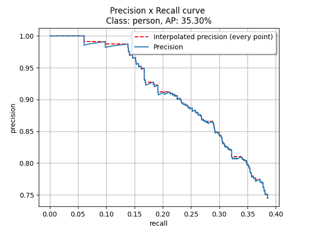
Finally after getting the precision recall values, we would be calculating the mAP(mean Average Precision) using 11 point interpolation technique. I have kept the default IOU threshold value as 0.5, which can be changed accordingly.
In short, this is how we calculate the mAP(mean Average Precision):
- Plot Precision and Recall curve from the values obtained.
- Calculate the mean Average Precision(mAP), using 11 point interpolation technique on the above Precision VS Recall graph.
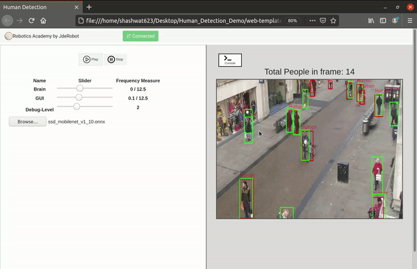
Benchmarking on the Oxford Town Center dataset
Next, I integrated the finished benchmarking code with the Human Detection exercise to obtain benchmarking statistics in real time on the Oxford Town Centre dataset, which we previously pre-processed. Here are some of the challenges faced during it’s integration:
- Including the whole code in the
exercise.pyfile would make it messy, so it was essential to break it down and include it as a dependency. For this reason I have just included aperform_benchmark()function in the exercise code, which synchronizes with all other dependencies for benchmarking without making a mess.
    def perform_benchmark(self):
        currentPath = os.path.dirname(os.path.abspath(__file__))
        acc_AP = 0
        validClasses = 0
        # Read txt files containing bounding boxes (ground truth and detections)
        # getBoundingBoxes() function is present inside benchmark.py
        boundingboxes = benchmark.getBoundingBoxes()
        savePath = os.path.join(currentPath, 'benchmarking/results')
        shutil.rmtree(savePath, ignore_errors=True)
        os.makedirs(savePath)
        # Create an evaluator object in order to obtain the metrics
        evaluator = Evaluator()
        # Plot Precision x Recall curve
        detections = evaluator.PlotPrecisionRecallCurve(
            boundingboxes,  # Object containing all bounding boxes (ground truths and detections)
            IOUThreshold=0.3,  # IOU threshold
            method=MethodAveragePrecision.EveryPointInterpolation,  # As the official matlab code
            showAP=True,  # Show Average Precision in the title of the plot
            showInterpolatedPrecision=True, # Plot the interpolated precision curve
            savePath = savePath)
        f = open(os.path.join(savePath, 'results.txt'), 'w')
        f.write('Average Precision (AP), Precision and Recall: ')

        # each detection is a class
        for metricsPerClass in detections:
            # Get metric values per each class
            cl = metricsPerClass['class']
            ap = metricsPerClass['AP']
            precision = metricsPerClass['precision']
            recall = metricsPerClass['recall']
            totalPositives = metricsPerClass['total positives']
            total_TP = metricsPerClass['total TP']
            total_FP = metricsPerClass['total FP']

            if totalPositives > 0:
                validClasses = validClasses + 1
                acc_AP = acc_AP + ap
                prec = ['%.2f' % p for p in precision]
                rec = ['%.2f' % r for r in recall]
                ap_str = "{0:.2f}%".format(ap * 100)
                print('AP: %s (%s)' % (ap_str, cl))
                f.write('\n\nClass: %s' % cl)
                f.write('\nAP: %s' % ap_str)
                f.write('\nPrecision: %s' % prec)
                f.write('\nRecall: %s' % rec)

        mAP = acc_AP / validClasses
        mAP_str = "{0:.2f}%".format(mAP * 100)
        print('mAP: %s' % mAP_str)
        f.write('\n\n\nmAP: %s' % mAP_str)
        f.close()
- Normal inference and benchmarking would be separate choices for the user, so a different function(
eval_dl_model()) to perform evaluation and saving the corresponding detections was needed. I wish I could include all the code for it here, but that would make this blog messy as I have already included a lot of code here. Please refer to theexercise.pyfile for that. - Implementing all this with the pre-existing code base of the exercise was a bit confusing and time consuming but it did work out in the end :)
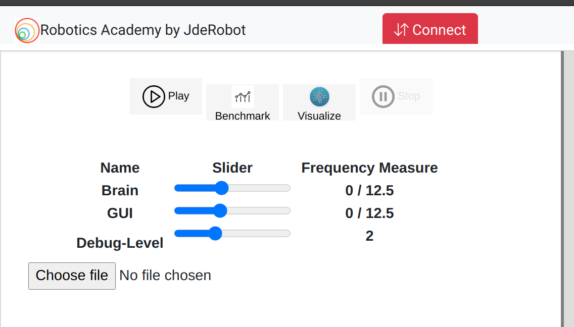
Added custom buttons and their functionalities for benchmarking and visualization
As of now there was no option to choose between inference, benchmarking and visualization features. I had hard coded everything while testing the separate features. As of now everything would just pop up on the screen. It was now time to implement the custom buttons on the front end for them and of course their corresponding functionalities in the front and back end.
- Play button - This was already included from before. This is used to perform inference in real time from the web cam input.
- Benchmark button - This is used to start performing benchmarking on the uploaded model as shown above.
- Visualize button - This is used to open the model visualizer after the model has been uploaded.